In order to transmit the bits over a physical channel they must be transformed into a physical waveform. A line coder or baseband binary transmitter transforms a stream of bits into a physical waveform suitable for transmission over a channel. Line coders use the terminology mark for “1” and space to mean “0”. In a baseband systems, binary data can be transmitted using many kinds of pulses. These many types of waveforms are there to satisfy different performance criteria in different scenarios! Each line code type has its own merits and demerits. The choice of line code waveform depends on operating characteristics of a system such as:
1. Bandwidth requirement: Line codes like NRZ-L require less bandwidth but have demerit of having DC level and bad synchronization.
2. Synchronization requirement: Line coding scheme like Manchester have good synchronization but require significantly higher bandwidth.
3. Receiver complexity: Complicated schemes obviously require more complex receiver adding to the cost.
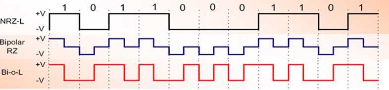
The input to the line encoder is the digital bit stream to be transmitted over the channel and output is a sequence of waveforms as a function of the input data bits. Here, we are going to present the Matlab simulation of Bipolar NRZ-L, Bipolar-RZ and Manchester-L schemes. In the figure below, we can see how a sequence of bits ‘10110001101’ is encoded as physical wave-forms by each of these schemes. For NRZ-L, a ‘1’ is represented as positive voltage +V during the whole bit duration while a ‘0’ is represented as negative voltage -V during the whole bit duration. In comparison for Bipolar-RZ, we see that in the middle of the bit +V and -V return to zero for ‘1’ and ‘0’, respectively. Bi-phase-L is another name for manchester-L scheme where we see the transition from +V to -V in the middle of bit for ‘1’ and a transition from -V to +V for ‘0’.

In order to simulate these waveforms in Matlab and compare their Power Spectral Densities (PSDs) we will need to represent these waveforms as discrete values/samples. In the case of our simulation, we are representing waveform corresponding to each bit as 10 samples. For example, for Bipolar RZ-L if the input bit is ‘1’, we will generate sampled waveform “V V V V V 0 0 0 0 0” at the output and in case of ‘0’ output will be “-V -V -V -V -V 0 0 0 0 0”. The complete source code is given as follows:
clear all;
close all;
%Nb is the number of bits to be transmitted
Nb=10000;
% Generate Nb bits randomly
b=rand(1,Nb)>0.5;
%Rb is the bit rate in bits/second
Rb=4;
%Since each waveform is represented by 10 samples so sampling
%frequency is 10 times the bit rate
fs=10*Rb;
NRZ_out=[];
RZ_out=[];
Manchester_out=[];
%Vp is the peak voltage +v of the waveform
Vp=5;
%Here we encode input bitstream as Bipolar NRZ-L waveform
for index=1:size(b,2)
if b(index)==1
NRZ_out=[NRZ_out [1 1 1 1 1 1 1 1 1 1]*Vp];
elseif b(index)==0
NRZ_out=[NRZ_out [1 1 1 1 1 1 1 1 1 1]*(-Vp)];
end
end
%Now we draw the PSD spectrum of Bipolar NRZ-L using Welch PSD
%estimation method
h = spectrum.welch;
Hpsd=psd(h,NRZ_out,'Fs',fs);
figure;
hold on;
handle1=plot(Hpsd)
set(handle1,'LineWidth',2.5,'Color','r')
%Here we encode input bitstream as Bipolar RZ waveform
for index=1:size(b,2)
if b(index)==1
RZ_out=[RZ_out [1 1 1 1 1 0 0 0 0 0]*Vp];
elseif b(index)==0
RZ_out=[RZ_out [1 1 1 1 1 0 0 0 0 0]*(-Vp)];
end
end
%Now we draw the PSD spectrum of Bipolar RZ using Welch PSD
%estimation method
h = spectrum.welch;
Hpsd=psd(h,RZ_out,'Fs',fs);
handle2=plot(Hpsd);
set(handle2,'LineWidth',2.5,'Color','b')
%Here we encode input bitstream as Manchester-L waveform
for index=1:size(b,2)
if b(index)==1
Manchester_out=[Manchester_out [1 1 1 1 1 -1 -1 -1 -1 -1]*Vp];
elseif b(index)==0
Manchester_out=[Manchester_out [1 1 1 1 1 -1 -1 -1 -1 -1]*(-Vp)];
end
end
%Now we draw the PSD spectrum of Manchester-L using Welch PSD
%estimation method
h = spectrum.welch;
Hpsd=psd(h,Manchester_out,'Fs',fs);
handle3=plot(Hpsd)
set(handle3,'LineWidth',2.5,'Color','k')
legend('Bipolar NRZ-L','Bipolar-RZ','Manchester-L');
hold off;
figure;
stem((1:Nb*10)/10,NRZ_out);
xlabel('bits-->');
ylabel('Amplitude (volts)-->');
title('Bipolar NRZ-L encoded bit stream');
figure;
stem((1:Nb*10)/10,RZ_out);
xlabel('bits-->');
ylabel('Amplitude (volts)-->');
title('RZ-L encoded bit stream');
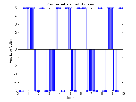
figure;
stem((1:Nb*10)/10,Manchester_out);
xlabel('bits-->');
ylabel('Amplitude (volts)-->');
title('Manchester-L encoded bit stream');
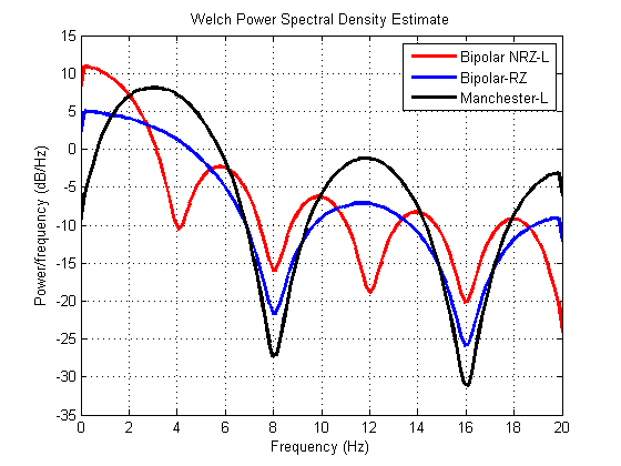
The PSD comparison of these Line Coding schemes is given as:
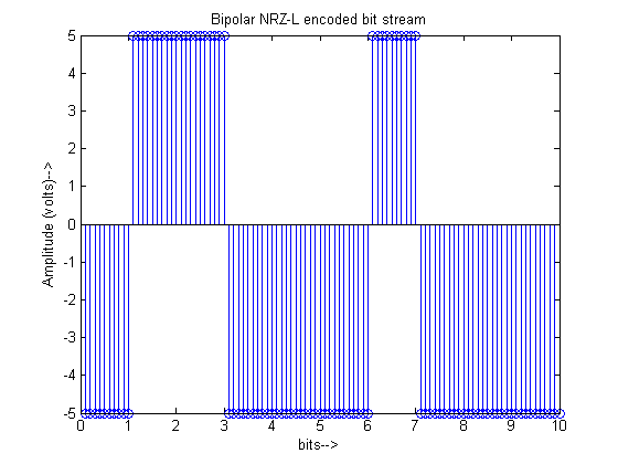
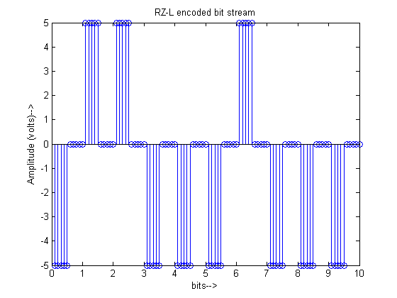
 For input bitstream of ‘01100010000’ the output of the different line coders is plotted as:
2 responses to “Matlab Simulation Of Line Codes And Their PSD Comparison”
thanks for this nice explination.
i would like to ask you about bi -phase-l. how we can compresse it, therefore, how we can do compression in Matlab.
thanks.
I consider something truly interesting about your website so I saved to fav. Fanchon Davon Oakley